Word-based analysis with song lyrics
2023 version: https://github.com/kahnwong/lyrics-analysis
I listen to a lot of music, mostly symphonic heavy metal. What's interesting is that in this genre, each album often has different themes, also each band focus on different topics in terms of lyrics. For instance, Nightwish focuses on nature, and their Imaginaerum album focuses on evolution. So I thought it would be interesting if I apply various text analysis methods to the lyrics, which resulted in this article. Github link here!
Techniques used
- tokenization
- stemming and lemming
- topic modeling
Import modules
from collections import Counter
import matplotlib.colors as colors
import matplotlib.pyplot as plt
import numpy as np
import pandas as pd
import seaborn as sns
from nltk import word_tokenize
## from nltk.corpus import stopwords
from nltk.stem import PorterStemmer
from sklearn.decomposition import LatentDirichletAllocation, NMF
from sklearn.feature_extraction.text import CountVectorizer, TfidfVectorizer
sns.()Import data generated from 01_get_data.py
In this step, I import raw data and convert raw year into a decade, for instance 1993 is in 1990s. I won't be doing analysis by decades, because in heavy metal it doesn't follow the trend much. But I include it here in case you are working on pop artists. In addition, the differences by year may not be that large, so it makes sense to see it in terms of decades.
df = pd.("lyrics.csv")
## dop song duplicates from the same artist
df.(subset=["artist", "title"], inplace=True)
## tokenize, remove stopwords, stemming and lemming
## stop_words = set(stopwords.words('english'))
with open("english.txt", "r") as f:
stop_words = [i.() for i in f.()]
ps =()
df["tokens"] = df.lyrics.(
lambda x: [
ps.(w)
for w in(x.())
if (not w in stop_words) and (not "'" in w) and (len(w) > 1)
]
)
## count words
df["word_count"] = df.tokens.(lambda x: len(x))
## count unique words
df["unique_word_count"] = df.tokens.(lambda x: len(set(x)))
## remove outliers
df = df[df.word_count > 10]
## set decade
df["year"] = df.year.(int)
df["1990s"] = np.(((1990 <= df.year) & (df.year <= 1999)), "1990s", None)
df["2000s"] = np.(((2000 <= df.year) & (df.year <= 2009)), "2000s", None)
df["2010s"] = np.(((2010 <= df.year) & (df.year <= 2019)), "2010s", None)
df["2020s"] = np.(((2020 <= df.year) & (df.year <= 2029)), "2020s", None)
df["decade"] = (
df["1990s"]
.(df["2000s"])
.(df["2010s"])
.(df["2020s"])
)
## drop unused columns
df = df.(columns=["1990s", "2000s", "2010s", "2020s"])
df| artist | album | title | lyrics | year | tokens | word_count | unique_word_count | decade | |
|---|---|---|---|---|---|---|---|---|---|
| 0 | Nightwish | Angels Fall First | Elvenpath | (In the sh | 1996 | ['shelter', 'shade', 'forest', ...] | 121 | 90 | 1990s |
| 1 | Nightwish | Angels Fall First | Beauty And The Beast | Remember t | 1996 | ['rememb', 'danc', 'share', ...] | 74 | 56 | 1990s |
| 2 | Nightwish | Angels Fall First | The Carpenter | Who are yo | 1996 | ['condemn', 'shine', 'salvat', ...] | 74 | 42 | 1990s |
| 3 | Nightwish | Angels Fall First | Astral Romance | A nocturna | 1996 | ['nocturn', 'concerto', 'candlelight', ...] | 69 | 68 | 1990s |
| 4 | Nightwish | Angels Fall First | Angels Fall First | An angelfa | 1996 | ['angelfac', 'smile', 'headlin', ...] | 68 | 49 | 1990s |
| 5 | Nightwish | Angels Fall First | Tutankhamen | As the sun | 1996 | ['sun', 'set', 'pyramid', ...] | 67 | 41 | 1990s |
| 6 | Nightwish | Angels Fall First | Nymphomaniac Fantasia | The scent | 1996 | ['scent', 'woman', '...'] | 29 | 28 | 1990s |
| 7 | Nightwish | Angels Fall First | Know Why The Nightingale Sings | What does | 1996 | ['fall', 'feel', 'boy', ...] | 49 | 47 | 1990s |
| 8 | Nightwish | Angels Fall First | Lappi (Lapland) | Part 1: Er | 1996 | ['erämaajärvi', 'kautta', 'erämaajärven', ...] | 63 | 54 | 1990s |
| 9 | Nightwish | Angels Fall First | Once Upon A Troubadour | A lonely b | 1996 | ['lone', 'bard', 'wander', ...] | 91 | 62 | 1990s |
Explore relationship
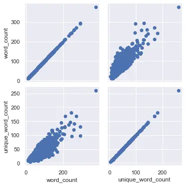
From this plot, I can see that there is a correlation between word_count and unique_word_count, that is, they go in the same direction. The higher the word_count, the higher unique_word_count and vice versa.
g = sns.(df[["word_count", "unique_word_count"]])
g.(plt.scatter)
Boxplot
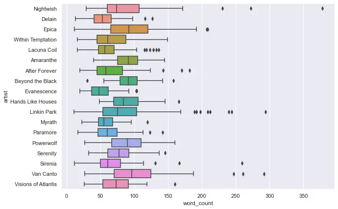
We can use either word_count or unique_word_count, since they go in the same direction, except the values from unique_word_count will be higher, but it is proportional to word_count
Boxplot represents data distribution in quartiles, in which the the box-y area is in middle of the distribution (think of a bell curve, the box-y area is right around the peak, padded a bit to left and right), and the line-y area is the left/right edge of the curve. The scattered points are outliers, meaning they are too different from the rest of the dataset.
From this figure, I can see that Nightwish has a very large outlier, seeing one data point is in 350 range. Myrath has the least words, and Linkin Park has the most. For Linkin Park, it can be attributed to the fact that their lyrics contain rap verses. As for Nightwish outliers, some of their songs contain very lengthy spoken parts.
plt.(figsize=(10, 7))
sns.(x="word_count", y="artist", data=df, orient="h")
Most common words
In this step, I count how many times a word occur per dataset, then plot a bar graph for each. For the bands I usually listen to, each album has a theme, so it's very probable that each album would have different set of most common words.
def word_vector(df):
########## make a list of all unique words
all_words = []
for i in df.tokens:
all_words.(set(i))
all_words = set(all_words)
########## make tf/idf
word_count = df.tokens.(lambda x:(x))
word_count = pd.(word_count.())
########## get sum for each unique word
wordcount_sum = []
for i in word_count.columns:
wordcount_sum.({"word": i, "count": word_count[i].()})
wordcount_sum = pd.(wordcount_sum)
wordcount_sum = wordcount_sum[wordcount_sum["count"] != 0]
wordcount_sum.(by="count", ascending=False, inplace=True)
##########
return wordcount_sum.(10)
## get wordcount for each group, this way the word_vector function is not getting messy
wordcount_group = []
################## adjust filters here
artist = "Epica"
group = "album" # album, decade
##################
df_temp = df[df.artist == artist]
for i in df_temp[group].():
chunk =(df_temp[df[group] == i])
chunk[group] = i
wordcount_group.(chunk)
wordcount_group = pd.(wordcount_group)
## plot
fig, axs = plt.(
len(wordcount_group[group].()), figsize=(13, 53)
) # adjust figure size here if it's too cramped
for index, i in enumerate(wordcount_group[group].()):
temp = wordcount_group[wordcount_group[group] == i]
axs[index].(temp["word"], temp["count"])
axs[index].(i)
From the above image, you can see that the top words don't vary much between albums. So I can conclude that Epica have a consistent lyric themes, but if you listen you can hear that their melody changes every album. For instance, in The Divine Conspiracy, it's very classical and oriental oriented, but in The Holographic Principle it gets heavier.
But that's only variations between albums from one artist. What if we do the same but with each artist instead?
wordcount_group = []
df_temp = df
group = "artist"
for i in df_temp[group].():
chunk =(df_temp[df[group] == i])
chunk[group] = i
wordcount_group.(chunk)
wordcount_group = pd.(wordcount_group)
fig, axs = plt.(
len(wordcount_group[group].()), figsize=(13, 80)
) # adjust figure size here if it's too cramped
for index, i in enumerate(wordcount_group[group].()):
temp = wordcount_group[wordcount_group[group] == i]
axs[index].(temp["word"], temp["count"])
axs[index].(i)
Whoops. Still more or less the same. But if you look carefully, Powerwolf stands out because their lyrical themes are werewolves and myths.
Topic modeling
So I change the tactics a bit by using topic modeling instead of seeing just the top words count. This way, the model and extract group of words that said to be the essence belonging to each cluster. I use both NMF and LDA here for comparison. Here, I tell the model to read lyrics from four artists, then try to group into clusters and finding main words from each, but I'm not telling it which document belongs to which artist.
def display_topics(model, feature_names, no_top_words):
topic_words = []
for topic_idx, topic in enumerate(model.components_):
print("Topic %d:" % (topic_idx))
topic = " ".(
[feature_names[i] for i in topic.()[: -no_top_words - 1 : -1]]
)
print("\t" + topic)
topic_words.(topic)
return topic_words
## define temp dataframe here
temp = df.(
'artist == "Visions of Atlantis" or\
artist == "Lacuna Coil" or\
artist == "Epica" or\
artist == "Nightwish"'
)
## define parameters
no_features = 1000
no_topics = len(temp.artist.()) # set album count as number of topics
no_top_words = 15
## create word matrix
tfidf_vectorizer =(
max_df=0.95, min_df=2, max_features=no_features, stop_words="english"
)
tfidf = tfidf_vectorizer.(temp.lyrics)
tfidf_feature_names = tfidf_vectorizer.()
print("========== NMF ==========")
nmf =(
n_components=no_topics, random_state=1, alpha=0.1, l1_ratio=0.5, init="nndsvd"
).(tfidf)
topic_words =(nmf, tfidf_feature_names, no_top_words)========== NMF ==========
Topic 0:
ll time life way light come live free just feel inside ve day let world
Topic 1:
love heart night wish forever hate soul dream oh art rest heaven need kiss lust
Topic 2:
away run far stay inside journey dream fade just wash felt destruction escape falling walked
Topic 3:
don know wanna want just feel say care hate goes cause liar let look reasonprint("========== LDA ==========")
lda =(
n_components=no_topics,
max_iter=5,
learning_method="online",
learning_offset=50.0,
random_state=0,
).(tfidf)
topic_words =(lda, tfidf_feature_names, no_top_words)========== LDA ==========
Topic 0:
distance don beautiful let today cold look guide read world way faith wish mind heart
Topic 1:
est tale feels talking drives wall wishmaster disciple bone mad searching free master apprentice sing
Topic 2:
love heart ll hearts time world fight let come night know shadows try eyes mind
Topic 3:
leaving ll healing endless sed died walk desire life nos ne moment die nostra likeFrom NMF, I can tell that:
- Topic 0 is Epica
- Topic 1 is Nightwish
- Topic 2 is Visions of Atlantis
- Topic 3 is Lacuna Coil
I think NMF performs better in this case 😆
There are some instances LDA performs better, but generally unless it's very obvious from the start, sometimes you use different models and see which performs best for a given dataset.